
Fire Escape! Malmo Collaborative AI Challenge
Summary of the Project:
Our project will aim to train an agent to complete a challenge map in the least number of steps. The challenge maps will consist of obstacles such as fire blocks and holes which the agent must learn to navigate and avoid obstacles only when necessary. In particular, we are interested in finding the minimum number of steps to complete a map without dying. The input for our agent will consist of the block type and obstacle locations on the map. The output will be the chosen movement of the agent. We will aim for the agent to take the shortest possible route during the challenge run using Q-learning and Deep Q-learning to gradually learn an optimal policy.
Approach
Since our project involves having an agent learn the optimal actions required to reach the goal, we decided that Reinforcement Learning was the best approach. In particular, we used the Q-Learning update function shown in Figure 1 to teach our agent to navigate the map safely. Q-Learning is an algorithm that teaches an agent which action to take given a state through rewards and punishments. Q-Learning uses a table of Q-values which is used to rate an action based on a given state and the value of the next best action. The learning rate will determine the degree of change to the Q-table per iteration. The discount factor determines how much future actions will impact the rating of the current action. For the basic implementation of Q-Learning, we defined our state space to be:
(size of the map * number of health states)
Figure 1: Q-learning Update Function
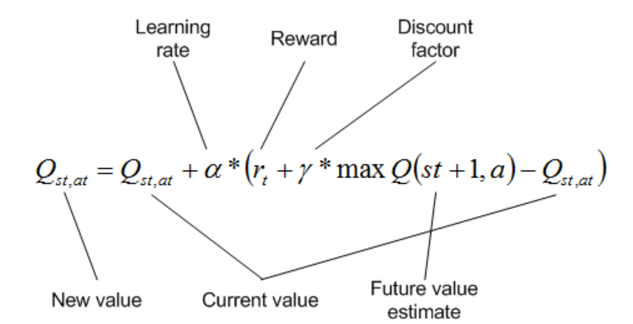
For the basic version of our algorithm, we kept the size of the map to be less than 25 blocks and 3 health states: full health, less than ⅔ health, less than ⅓ health. For our action states, we allow the agent to have four different actions: forward, backward, left, and right. This would produce a Q-table with the size:
(map size * number of health states * number of action states)
In our project we have a max Q-table size of: 2534 = 300
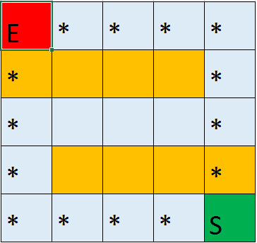
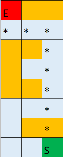
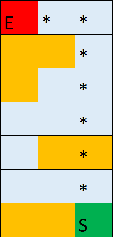
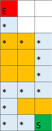
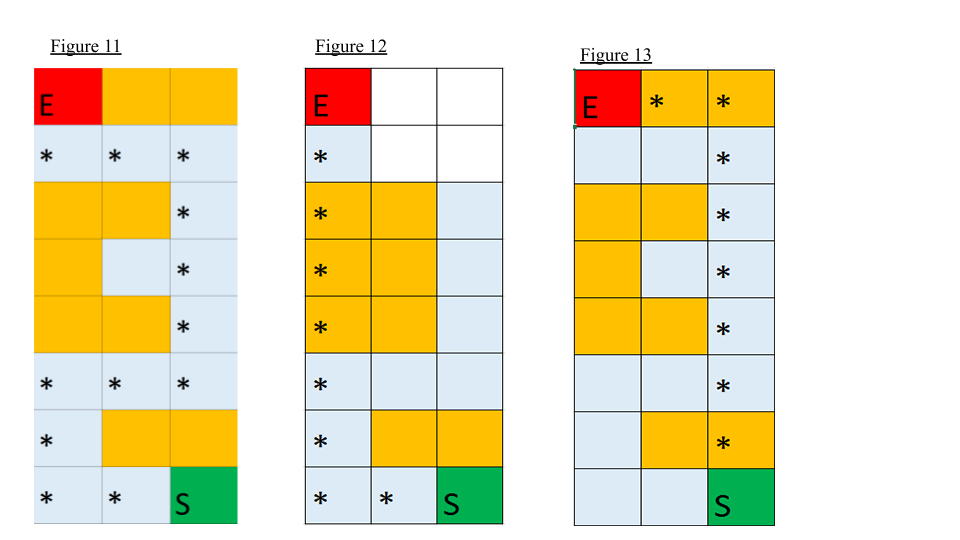
The * symbol on the maps represent the optimal path to the goal block.
Map 1
Map 2
Map 3
Map 4
For each action the agent completes, a positive reward or negative reward will be given based on the resulting state the agent is in. The reward function we implemented uses three main factors to calculate the reward given for an action:
1. Distance from goal block calculated using Dijkstra’s Shortest Path
2. Amount of health remaining
3. The agent’s survival after an action
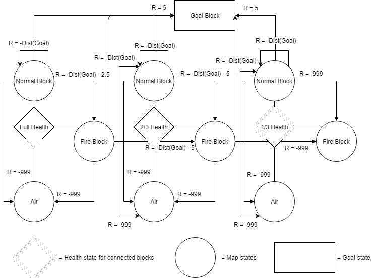
The main heuristic we used to determine the reward given to an agent is the distance from the goal block. The farther away from the goal block, the lower the reward given. This will incentivize the agent to get closer to the goal block with each action. A reward will also be given when the agent reaches the goal. During the agent’s adventure learning the map, if the agent happens to die from falling or fire, a large negative reward will be given to deter the agent from committing the same action in the future. The negative reward given when stepping on fire will be calculated based on the health state the agent is in. When the agent is max health, a small negative reward is given for stepping on fire. This is to encourage the agent to go through fire if it can shorten the distance from the goal significantly. As the agent’s health decrease, the negative reward will increase to deter the agent from dying to fire damage. A diagram of the Markov Decision Process is shown in Figure 2:
Figure 2
To ensure that the agent visits as many states as possible, a randomness factor is added when the agent picks its action. There is a predetermined percentage chance (10% in our project) for the agent to randomly choose an action. This randomness factor decreases linearly each time the agent completes the map.
Evaluation
Our evaluation method is separated into two parts: the quantitative measures and qualitative measures. For our quantitative measures, we kept track of several key variables during runs to determine that the agent is functioning as intended and accomplishing its goal. For our qualitative measures, we focus on gauging whether the agent can find the optimal shortest path. If there are multiple optimal paths, the agent will choose the path that maximizes health.
Quantitative Measures:
The quantitative evaluation of our algorithm is based on these three metrics:
1. Reward values per episode
2. Number of moves per episode
3. Number of successful episodes
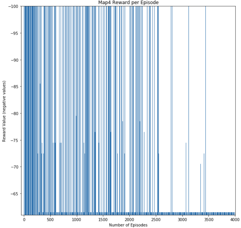
These three metrics help us measure the agent’s performance by measuring if it is continuously learning and improving the optimal path it knows. The main metric we use to determine if the agent is learning is the reward value per episode. By keeping track of this metric, we can gauge if the agent is improving on the action it chooses at each state. The reward value per episode indicates the quality of the path chosen in that episode. An episode where the agent dies or makes several inefficient actions will result in a low reward value at the end of the episode. An episode where the agent optimizes its action and chooses the optimal path will result in the highest reward value. Our main goal is to have the agent continuously achieve the maximum reward value per episode at the end of a training session. The Figure 3, Figure 4, Figure 5, and Figure 6 below shows the reward value per episode in one training session. As it can be seen in the graphs, at the beginning of the training session, there is a large variance in the reward value per episode. As the agent progresses through the session, the reward values would converge to the highest reward value obtainable in a particular map. This shows that our agent has learnt the optimal path for that map.
Figure 3: Map1 Reward Per Episode
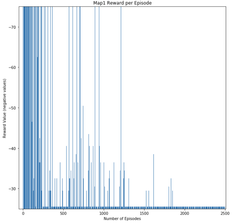
Figure 4: Map2 Reward Per Episode
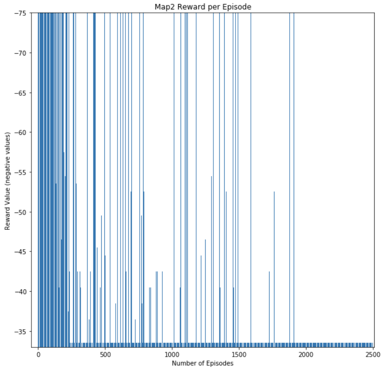
Figure 5: Map3 Reward Per Episode
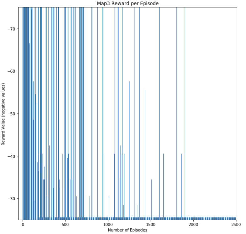
Figure 6: Map4 Reward Per Episode
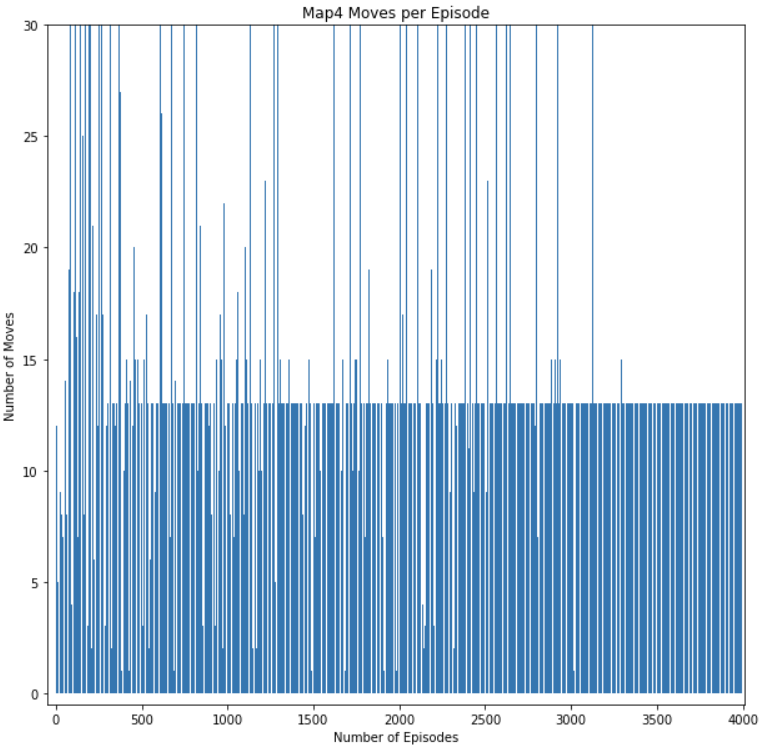
The metric number of moves per episode and number of successful episodes lets us gauge if the agent is successfully learning to avoid lethal obstacles. As the number of episodes increase, the number of moves per episode and successful episodes should start to increase also. This is because the agent should start rating actions that would cause it to fall off the map or burn to death to have high negative rewards. As a result, the agent should survive on the map longer and complete maps more consistently as it completes more episodes. This can be seen from results of the training session of our agent in Figure 7-10. As can be seen from Figure 7 and Figure 8, the graph shows that the rate of increase for the number of successful episode increases linearly at the end, meaning every episode is successful. In the beginning, the graph shows a much slower increase indicating that it was failing most of the early episodes. In Figure 9 and Figure 10, you can see that the number of moves per episode is very small in the beginning due to the agent dying early on in its episode. The number of moves increases significantly in the middle as the agent starts learning to avoid lethal moves while also exploring the map to find the optimal path to the goal. You can see the number of moves converge to a stable number at the end because the agent is starting to find the optimal path to the goal, which requires less moves.
Figure 7: Map1 Success per Episode Graph
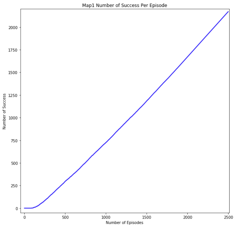
Figure 8: Map2 Success per Episode Graph
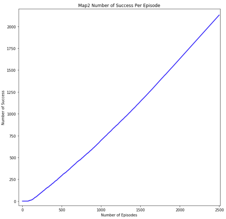
Figure 9: Map3 Moves per Episode Graph
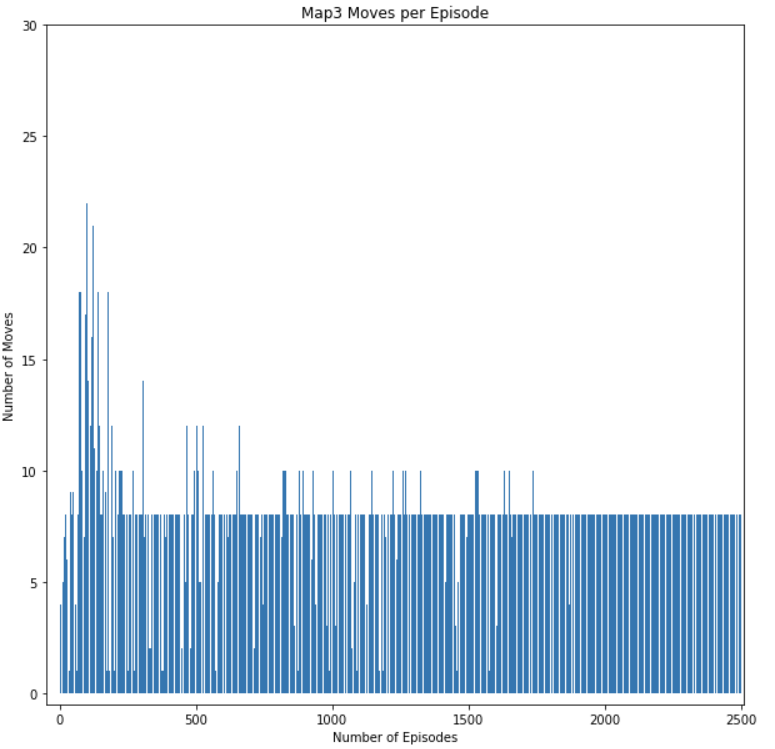
Figure 10: Map4 Moves per Episode Graph
Qualitative Measures:
The goal of our project is for an agent to learn the optimal path from a start block to a goal block while avoiding obstacles if necessary. To judge whether our agent accomplished this task, we used these three qualitative measures:
1. Whether path found is the optimal path (agent’s error rate)
2. Whether agent can complete map without dying
3. Amount of health upon reaching goal
Our main qualitative measure is whether the path found is optimal. The optimal path is defined as a path to the goal that takes the least amount of moves necessary while the agent stays alive. The agent can take damage along the path as long the damage taken would reduce the number of moves needed and does not kill the agent. To evaluate whether it can learn the optimal path, we created several test cases with a predetermined optimal path that we can compare to the path the agent learnt. The maps are specifically designed so that it will effectively test whether our agent can complete our qualitative measures. There are paths that result in no damage being taken but also takes slightly more moves (Figure 11), paths that kill the agent but result in less moves (Figure 12), and paths that would result in unnecessary damage being taken (Figure 13).
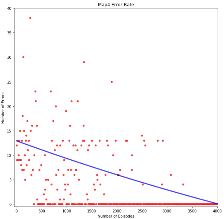
To evaluate the path the agent learns over a training session, we used the error rate metric. The error rate of the path an agent chooses is the number of moves that differ between the agent’s path and the optimal path. If an agent dies before reaching the goal block, the error rate would reflect that by calculating the difference between optimal number of steps and steps achieved. Figure 14, Figure 15, Figure 16, and Figure 17 shows the graph of the agent’s error rate versus number of episodes for each map. We can see that after several hundred episodes the error rate eventually converges to zero, meaning the agent has successfully found the intended optimal path. This shows that the agent has successfully completed the goal of our project.
Figure 14: Map 1 Error-Rate Graph
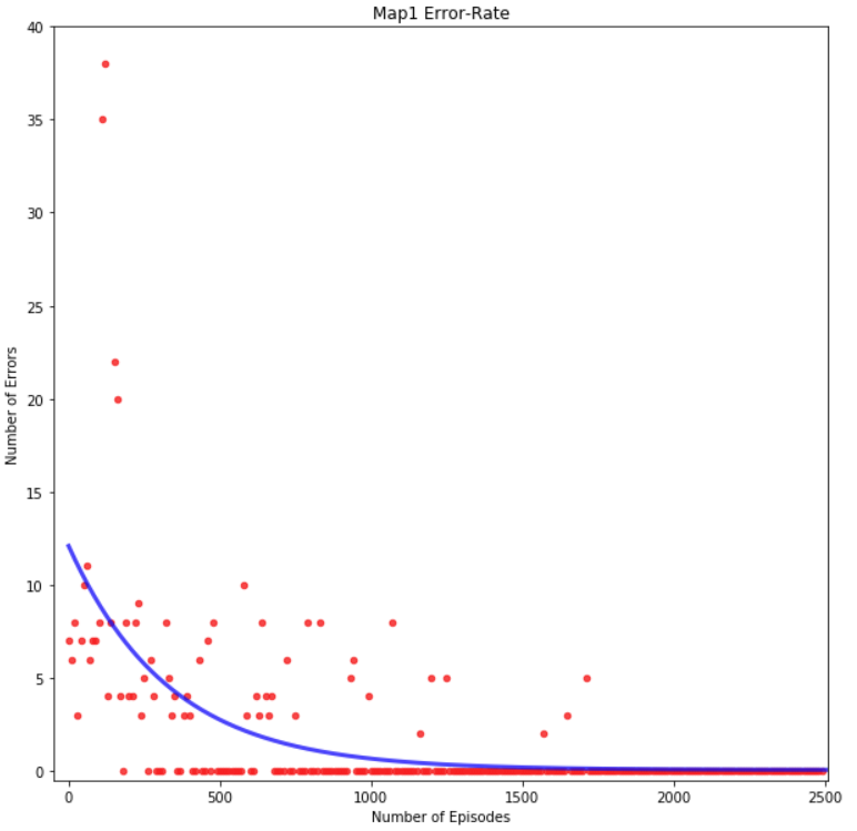
Figure 15: Map 2 Error-Rate Graph
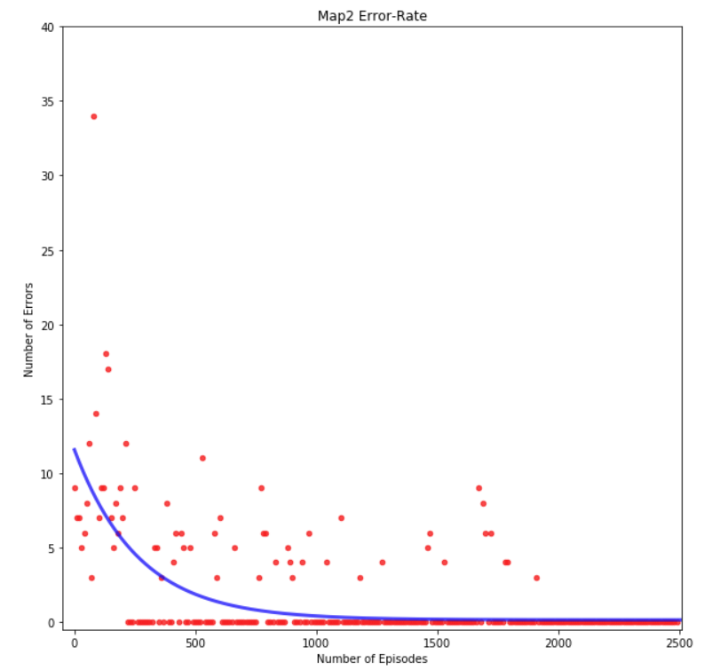
Figure 16: Map 3 Error-Rate Graph
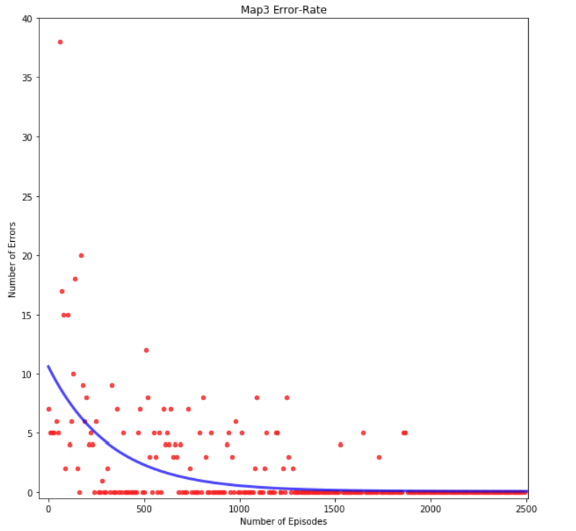
Figure 16: Map 4 Error-Rate Graph
Furthermore, to ensure that our agent is learning the optimal path, we included the graphical representation of the Q-table shown in Figure 17 indicating the improvement in path the agent learns. Each square in Figure 17 represents each block on the map. The blocks with red backgrounds represent fire blocks, while the black background represents normal blocks. The large white circle in the center of the block is the current agent’s position and the four small circles in each block represents the resulting Q-value of each direction from that particular block. Red small circles mean that the Q-values for those direction results in low rewards, while green small circles means that Q-value for those direction results in high rewards. As we can see in Figure 17, the Q-table will eventually show the optimal path that the agent learns.
Figure 17: Graphical representation of Q-table
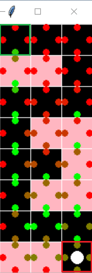
Green Outline = Start Block
Red Outline = End Block
Remaining Goals and Challenges
Remaining Goals:
Within the upcoming weeks, we have two main objectives we want to complete. Our first main objective is to implement real-time health states that would let an agent consider an action based on its current health state. Currently, our agent only considers three different health states (full health, ⅔ health and ⅓ health), which limits the versatility of the agent in certain scenarios. By tracking only three health states, the current algorithm may potentially only find a local maxima instead of the global maxima. Having a real-time health state would allow the agent decide on actions based on its current health percentage which may improve the versatility of the agent. This will most likely allow the agent to find solutions to more challenging maps that the our prototype agent could not.
Furthermore, with our current implementation of health-states we are exponentially increasing our state space based on the number of health states we decide to track. If we were to increase the number of health state being tracked, it would require a large amount of episodes for it to converge on larger maps. A possible solution to this problem would be to implement Q-Network Learning which would allow us to use multi-layer neural networks to actively track health-states.
Our second main objective is to implement jump as another action available for the agent to use to avoid obstacles and potentially find a shorter path. By implementing jump it would allow our agent to have another degree of freedom which opens up many new paths that it could not find with only the four current actions. Implementation jump would also allow the agent to solve maps with different elevation levels. This would give our agent another level of versatility.
Challenges:
There are several challenges that we anticipate as we attempt to implement Q-Network Learning and the jump action. Firstly, implementing jump would cause our current reward heuristic to no longer be completely valid. Our current heuristic relies on Dijkstra’s shortest path algorithm which calculates distance based on blocks that are walkable. When jump is implemented, then the shortest path available would no longer only be on walkable paths, which would cause Dijkstra’s to estimate the reward incorrectly. Thus, we need to improve the step cost function to properly account for having the jump action available. This can be done by reworking our heuristic either by changing it or not relying on a heuristic. With further testing, we should be able to construct an effective heuristic.
Secondly, implementing the Q-Network Learning would also be a challenge as that would requires learning how to implement the algorithm while also changing our existing functions. We would need to update most of our reward function to dynamically change the reward depending on health-states. Furthermore, we would also need to optimize the Q-Network Learning we implement.
Given our experience so far, we should be able to implement Q-Network Learning with sufficient testing, documentations and tutorials. It would mainly require time for our team to learn the intricacies of Q-Network Learning.
Resource Used
- Q-Learning
- https://medium.freecodecamp.org/an-introduction-to-q-learning-reinforcement-learning-14ac0b4493cc
- Malmo tutorial6.py
- https://www.youtube.com/watch?v=79pmNdyxEGo
- Figure 1: https://developer.ibm.com/articles/cc-reinforcement-learning-train-software-agent/
- Deep Q-learning:
- https://medium.com/emergent-future/simple-reinforcement-learning-with-tensorflow-part-0-q-learning-with-tables-and-neural-networks-d195264329d0